Arange demo with wave

Wave Propagation

A wave function is defined as

$$Y = A \sin(\omega t + kx)$$

Differential equation

$$\large{\frac{\partial^{2}U}{dt^{2}} = c^{2}\frac{\partial^{2}U}{dx^{2}}}$$

import numpy as np
import matplotlib.pyplot as plt
import seaborn as sns 
sns.set()

• Define Amplitude, angular frequency, wave vector

amp = 1.0
freq = 1
w = 2*np.pi*freq #angular frequency
k = 2*np.pi #wave vector

• Calcualte frequency, weblength and velocity

wave_length = 2*np.pi/k
velocity = freq*wave_length
(freq,wave_length,velocity)

(1, 1.0, 1.0)

Plot the different configuration of wave motion

xs = np.arange(0,5,1/20)
ts = np.arange(0,5,1/20)

len(xs),len(ts)

(100, 100)

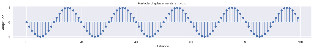
1. Experiment: Plot the particle displacement keeping time fixed

When we fix the time, it is a photograph of the wave motion at specific time t0. It can be represent as

$$Y = A \sin (kx + \phi_{0})$$

A special case is closed vibrating string

plt.figure(figsize = [18,2])
t0 = 0.0
y = amp*np.sin(w*t0 - k*xs)
plt.stem(y)
plt.xlabel("Distance")
plt.ylabel("Amplitude")
plt.title('Particle displacements at t=' + str(t0))

Text(0.5, 1.0, 'Particle displacements at t=0.0')

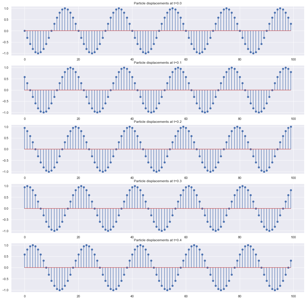
plt.figure(figsize = [18,18])
t0s = [0.0,0.1,0.2,0.3,0.4]
for i,t0 in enumerate(t0s):
    plt.subplot(len(t0s),1,i+1)
    y = amp*np.sin(w*t0 - k*xs)
    plt.stem(y)
    plt.title('Particle displacements at t=' + str(t0))

plt.show()

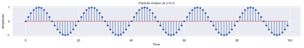
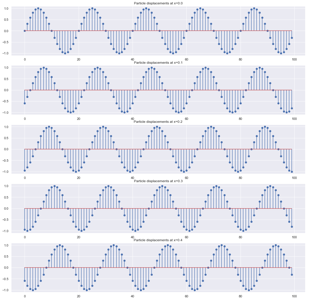
2. Experiment: Plot the particle displacement keeping position fixed

When we fix the position and look at a single particle displacement, it behaves like a harmonic oscillator. It can be represent as

$$Y = A \sin (\omega t + \phi_{0})$$

A special case is harmonic oscillator

plt.figure(figsize = [18,2])
x0 = 0.0
y = amp*np.sin(w*ts - k*x0)
plt.stem(y)
plt.xlabel("Time")
plt.ylabel("Amplitude")
plt.title("Particle motion at x=" + str(x0))

Text(0.5, 1.0, 'Particle motion at x=0.0')

plt.figure(figsize = [18,18])
x0s = [0.0,0.1,0.2,0.3,0.4]
for i,x0 in enumerate(t0s):
    plt.subplot(len(x0s),1,i+1)
    y = amp*np.sin(w*ts - k*x0)
    plt.stem(y)
    plt.title('Particle displacements at x=' + str(x0))

plt.show()

---

Animation 1D

Wave propagation in 1D

Next Step:

Wave Propagation in 2D (numpy meshgrid)